By Adam Wolf, Eion co-founder and Chief Innovation Officer
In my closing weeks of grad school I got to study at the Santa Fe Institute, and it was something of an epiphany. I had spent a significant portion of my time in grad school studying the branching patterns of trees, what they call allometry, as a way to understand what the Earth looks like from space. The pre-eminent authors of this work were at SFI, Geoffrey West and Brian Enquist, and they derived all sorts of equations that told you exactly what the surface area of a twig ought to be, based on the trunk diameter.
I spent grad school going deep into How – – how do I measure this? how do I simulate this? how does evaporation from grassland change the cloudiness of the sky above? And when I looked at equations, I was looking for How. What SFI introduced me to was Why. An equation isn’t there to make it easy to code something up, an equation is there to tell you why nature takes that expression at all. I bathed in (and nearly drowned in) this Why at the EEB department at Princeton and found that How rather more suits my skills (I am not a bona fide mathematician).
One of the lasting imprints of Santa Fe Institute is that the same math that tells you how trees grow also describes how cities evolve, and even how innovations are created and refined. Theory helps you imagine things that don’t yet exist. J Doyne Farmer, who was profiled in Gleick’s book Chaos for his work on clouds and turbulence at Los Alamos, landed at SFI where he was profiled by a McKinsey consultant in Origins of Wealth for applying this work to overturning economics. When I visited, he and his collaborator Jessika Trancik were busy trying to understand Learning Curves – which you probably know better as Moore’s Law. Learning Curves are really important for us, because they describe how things that are impossibly expensive now (like carbon dioxide removal) become affordable in time. We need that!
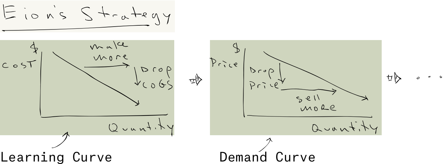
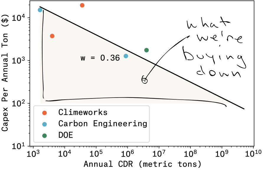
Klaus Lackner wrote a paper not long ago on “buying down” the cost curve for Direct Air Capture (link). He overlapped with Farmer at Los Alamos, I can only guess that he followed this work at SFI. The analogy he drew was with solar power, that as the installed base went up, the marginal cost went down:
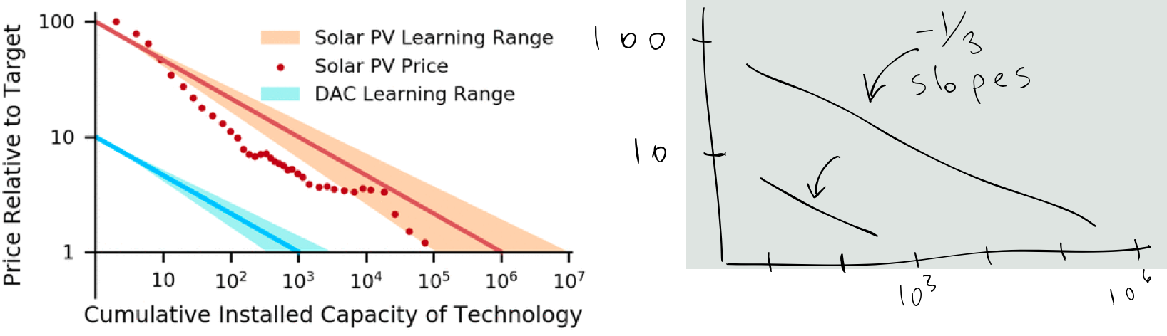
Lackner’s argument was not very different than Stripe’s argument: the desirable unit costs of a mature industry reflect the investments made in a nascent industry, when the unit costs are outrageous. Lackner skipped over the capex part of DAC, which dramatically improves the palatability of his results, but still the logic makes sense as far as the pro-social outcome. My question though is: Why that learning curve? Why the -1/3 slope? Is that good? Can we do better?
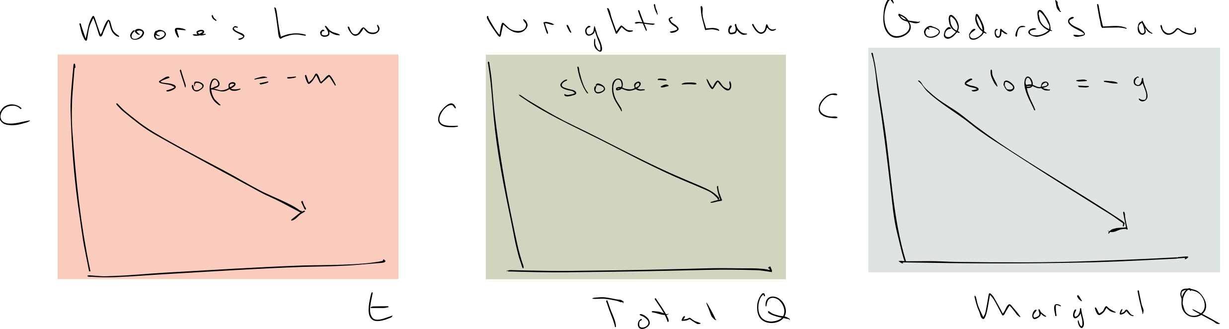
Theory: Wright’s Law, Moore’s Law, Goddard’s Law, etc
In 2013, Farmer and his colleagues published a piece on the theory of learning curves more generally, showing that Moore’s law (decrease in costs over time) is related to Wright’s law (decrease in costs with the installed base), and Goddard’s law (exponential increase in production over time). The short story is that w = m/g, which is actually a pretty stellar result. All these learning curves are different aspects to the same law.
Conveniently for us, they stockpiled all these learning curves and added them to a database that is maintained till this day. It turns out that the photovoltaic example that Lackner pulled as inspiration for DAC’s learning curve is nowhere close to ideal. Solar PV is better than the learning curve for postwar beer production in Japan (!), and on par with many technologies in energy, but the technologies that define our modern world, like transistors and hard drives, have learning curves of 0.7 and above.
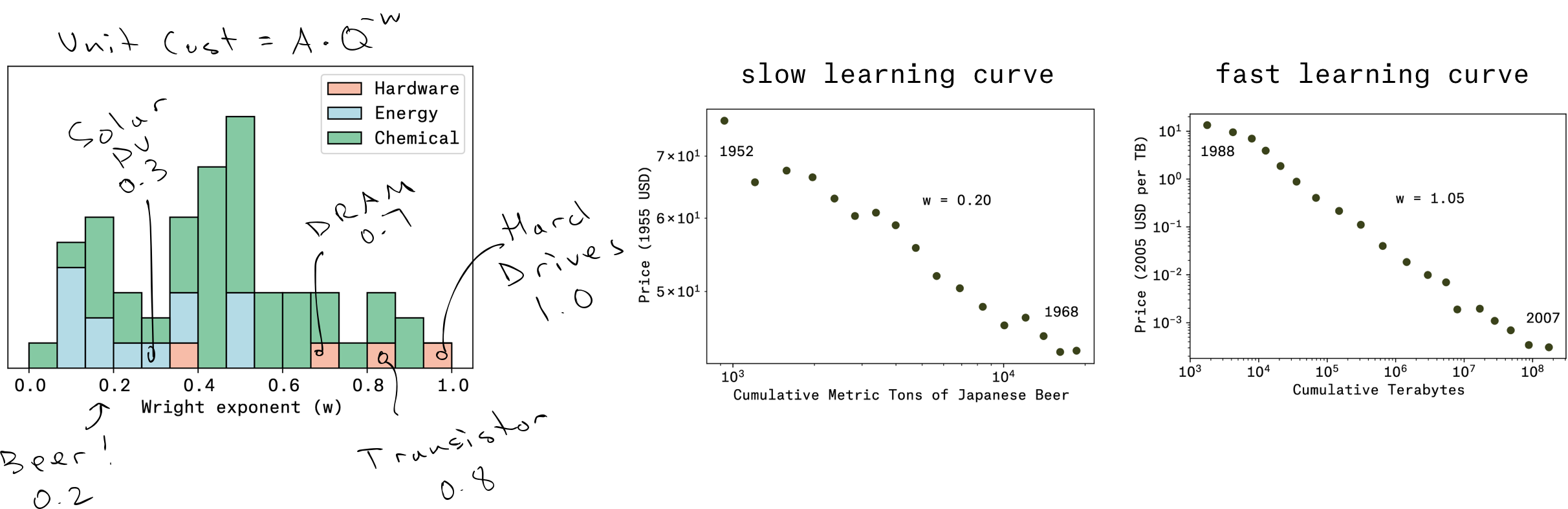
In fact, that exponent of 1.0 for hard drives is worth calling out for being essentially perfect – – it means “zero marginal costs”. This was driven home to me recently when we were booking freight to bring olivine over from Norway. We could move 10,000 tons for some cost – – or we could move 20,000 tons for the identical cost. In other words, cost times quantity is a constant. Rearrange, and you get that exponent of 1 . . . the Holy Grail of learning curves!

Learning curves for CDR
Within CDR, learning curves hold a special place, because in some sense we know the answer we want to get: $100 per ton of CO2. This is the metric established by the DOE (link), it is the metric established by Stripe in their first purchases (link). It is the industry’s North Star, and for Eion we hold it in our head as the cost where demand for permanent, verifiable CDR is unlimited. Thus, the learning curve is considered a first-class member of a CDR technology’s attributes (link), alongside basics like life cycle analysis, economic leakage, and additionality.
The people who take learning curves most seriously are in Direct Air Capture, in part because they are smart engineers who love using math to solve a problem, but in part because the current costs raise serious eyebrows. Let’s take the cost of capex.
- Climeworks’ Orca plant took $15M for a 4K ton per year (tpy) capacity => $3750/annual ton (link or link or link)
- Climeworks’ Mammoth plant uses $627M in equity to build a 36K tpy capacity => $19,592/annual ton (link)
- Carbon Engineering’s Newport plant cost $25M and removes 4.5tpd => $15,220/annual ton (ce)
- Carbon Engineering’s 1M tpy plant is estimated to cost $1126M => $1276/annual ton (link)
- DOE’s DAC Hubs is allocating $7B for 4 hubs each removing 1M tpy => $1750/annual ton (link)
Plot out that learning curve, and the prediction is that we’ll get to $100/t of capex when we’re producing around 5GT of CDR per year. Between now and then we’re paying 10 to 100x that amount, just to get better at building the capital equipment. Holy smokes! I don’t know if that’s a trillion dollars or just many billion dollars, but it’s still going to require sovereign wealth. I don’t quibble with other folks’ well reasoned analysis of pathways to reduce DAC opex as well, other than to say that these costs are also in the hundreds of dollars range, and also have a learning curve in the 0.3-0.4 range (it looks a lot like the energy sector), so those will also take years to reach $100/t.
Learning curves for ERW
I believe that all of our stakeholders want and need for CDR companies to be run as profitable businesses. Say we’re doing 10M tpy in 2030, and say we get our costs down to $100/t, then that’s a billion dollars of working capital. Nobody gives you terms for that kind of risk without knowing that your business makes sense. So indulge me for adding our own overhead costs into the learning curve. Last year we spent $2,032,402 overhead and removed 500 tons of CO2. This year (2023), our overhead doubles, to $4,366,899, but our production increases 20x to 12,500 tons. Next year (2024) our overhead comes up slightly, to $4,741,404, but our production increases another 20x, to 250,000 tons. I’ve heard our rock dust called magic, but the real magic is that you can increase production by orders of magnitude, while barely increasing costs. That is a learning curve of 0.87 . . looks like Silicon Valley type growth! Somewhere between transistors and hard drives. And so we’re clear, I could be off by like double on my overhead costs in 2024 and still we’re good.
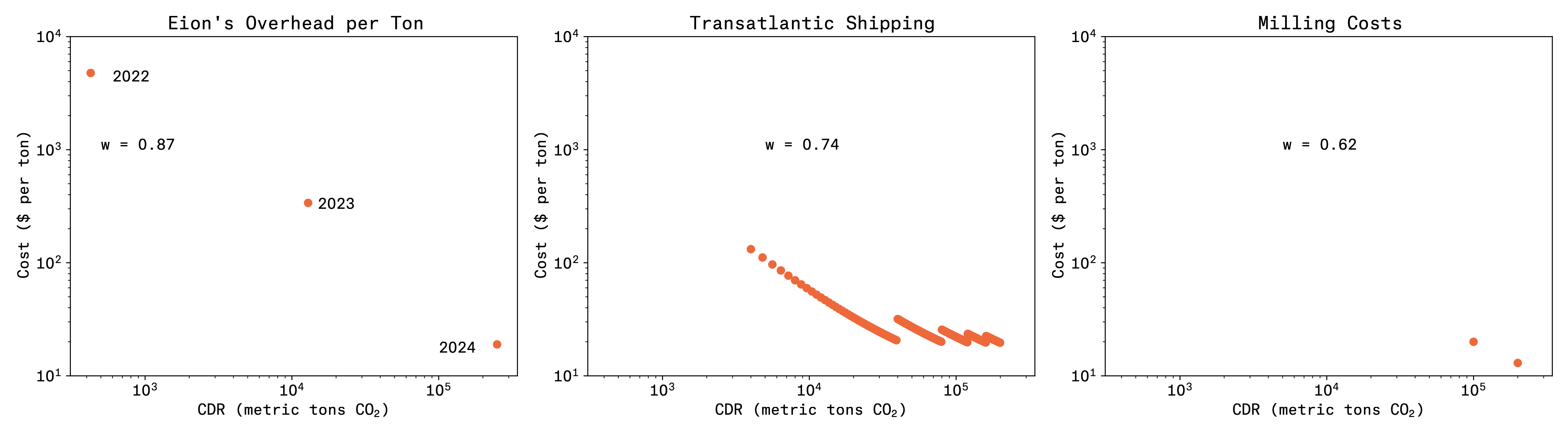
We’re able to achieve this because we are leveraging old industries. This is some real American Dynamism stepping up here. Overseas transport is already very optimized. Last mile trucking is optimized. Rock pulverizing is very optimized. In fact, you almost can’t see the dots on the milling capex costs, because they barely register on the chart, in the low double digits per annual ton. The opex for that mill is around there as well. In other words, the expense to “buy down” the costs for ERW are in the low single digit millions of dollars.
Now, within ERW, you might wonder how different feedstocks affect carbon prices. The following insight is not altogether deep, but I find it useful. The breakeven price comes down to the COGS divided by the mineral potential, the intrinsic capability of the mineral to remove carbon dioxide. (You should net this of emissions in the process, which are about 0.05 to 0.2 depending on the supply chain.)
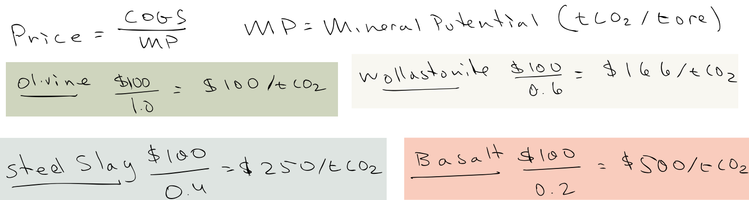
What you should draw from this is that ERW on its worst day performs better than many CDR technologies at their apotheosis. What’s more, I think you can start working on some of these numbers, e.g. by shortening the supply chains for basalt, which drop the COGS while raising the net CDR … $50/0.3 = $150, which is not bad. Which is to say these too are amenable to learning.
Costs of MRV
You can ask (people do it all the time!) where the costs of MRV show up here, because they are famously challenging to the economics of soil organic carbon markets. At a relatively high density of samples (1 per ha) we estimate around $20/tCDR, including sampling and lab analysis. Certainly that can be improved with refined sample design, both within and across fields, but the takeaway is that we should be focused on mass production first and foremost, so we can reach the 250K tpy milling capacity that is at the heart of making CDR affordable. That said, you can expect another Eion Explainer on sample design and MRV later!
As always: reach out for questions, comments, positivity: hello@eion.team